
The Dilemma
It’s no secret that I’m all about Modeling Instruction. While I don’t necessarily follow their curriculum to the “T”, the ideas behind it undoubtedly form the backbone of almost everything I do in my class. And I definitely use a fair share of their worksheets and labs almost verbatim.
The basic idea behind modeling is that all the equations, rules, laws, etc. that are typically delivered to students and expected to believe a priori are instead derived and discovered through a series of paradigm labs performed at the beginning of an instructional unit. This works great when you’re rolling balls down ramps or swinging pendulums, but it’s much more difficult (if not impossible) to this with things like Gauss’ Law or Electric Flux given even my very well funded equipment budget.
Thus, my dilemma. I’m teaching AP Physics C: Electricity and Magnetism for the first time this year, and I was terrified that I’d be reduced to mostly lecturing. I hate lecturing. My kids hate it, especially given that I had them last year. They’ve got expectations of what “Physics with Mr. Register” is like. And it just doesn’t work. Thankfully, desperation is a great motivator for me, and I think I’ve stumbled on to some excellent alternatives.
I won’t pretend to have all the answers right now, but things are turning out quite differently than I planned. The next two three posts will be two different paradigm “lab” ideas that I’m using to have students invent the concept of electric flux and to derive the simplest case of Gauss’ Law.
Where They’re At
My students have just finished working through deriving the electric field due to a thin ring, thin disk, and a half-circular ring the brute-force way:

Which is terrible, even for the most symmetric of situations (well, I think it’s super cool…). I’ve got my reasons for them doing this… but that’s for another post.
So at this point they’re aching for something simpler.
Electric Flux
We start with a quick review of field lines, in particular that the density of field lines at any particular point corresponds to the field strength. I then draw field lines for a point charge on the whiteboard and draw a few concentric circles around the charge.
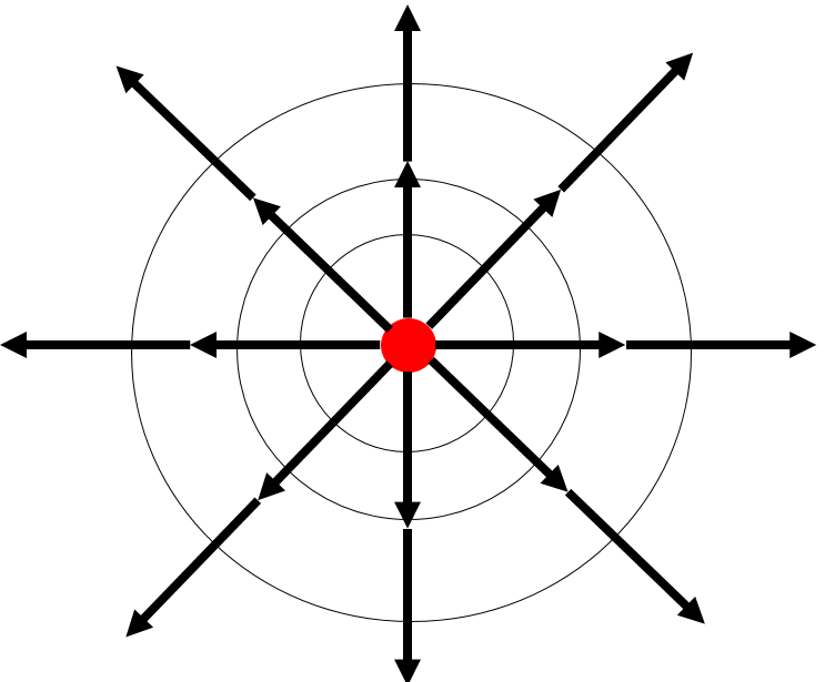
When prompted with How does the density of field lines change as the radius of these imaginary circles increases?, they quickly reply that the density decreases, which means that the field strength also decreases. Which is nothing new because we’ve been dealing with electric fields for 2 weeks now.
I then tell them that we’re going to examine the relationship between the area of these imaginary circles and the density of field lines within that circle, i.e. the field strength. Unfortunately, my only response to the question Uhh… why? is that they should trust me because it will take the nasty integral away. And because why not?
Except that we’re going to do it in 3D with the surface area of a sphere to better model reality, us living in a 3D world.

Instead of setting this up as an actual experiment, I explain that we’re going to put our theoretical physicist hats on.
They’re tasked with calculating the electric field strength of a 1 nC point charge at a distance of 1 to 7 m (in 1 m increments) along with the surface area of the accompanying sphere.
 Once they’re done with their calculations, they dutifully jump to graphing the data:

Linearizing and slope finding occurs, and then they generate the following equation:

After some discussion as to the meaning of the slope, students come up with essentially the definition for electric flux: the “amount” of electric field penetrating a given area. Then some rearranging and symbol assigning, and we’ve come up with a (very limited) mathematical definition of electric flux.

I also pose some additional, fairly standard follow-up questions:
- How does the flux change as the field strength increases and decreases? The area?
- How does the field strength change as the flux increases and decreases? The area?
Nothing very difficult at all for students in AP Calculus BC, but still important to discuss.
What’s Next?
We need to now generalize the equation for electric flux to include the pesky “only the perpendicular parts of the field are important” condition. I’m still figuring out how to have them arrive to that conclusion… but my current idea is to pose the following question: Why did I choose a sphere? Why not some other shape? Hint: think about symmetry.
Ideally, they’ll see the spherical symmetry of the situation and that will shed some light on why the fact that the field lines are perpendicular to the surface of the sphere at every point is important.
After a day or two whiteboarding with this new idea, I’ll ask students to investigate the relationship between the flux and the charge enclosed within the spherical surface, which will yield the simplest case of Gauss’ Law.
But I’ll wait to post about that once I get there. Until then, if you’ve got any ideas on how to improve on this, please share!

Trevor, great E&M posts! For this one, do you have the students use a simulation and collect the data themselves or you give them the data. Thanks!
Thank you!
If anything, I’d call it a “manual simulation”? At this point, they know how to calculate the field strength and direction due to single point charges, so I have them do that for a variety of distances from a 1 nC charge. Then, they calculate the surface area of a sphere for those same distances from the charge and plot field strength vs. surface area.
The downside here is that there’s no justification (to them, anyway) for why we’re calculating the surface area of an imaginary sphere versus, say, any other shape. They don’t get to see all the symmetry advantages until we get to the integral form of Gauss’ Law.
Now that I’m thinking about it, I wonder if this could also be done using one of the Phet sims? Definitely going to look into that for next year.
Thank you.
Perhaps creating one with Geogebra? Like these ones: http://ophysics.com/index.html